Decision Tree

Name: Decision Tree

Category: Supervised prediction - classification

Introduction

Just like the naïve Bayes algorithm, decision trees are a very popular machine learning technique that most practitioners (novice and expert) usually apply to their data early on in the analysis process. However, the reasons for choosing them often to differ somewhat from why you might decide to use naïve Bayes. Suppose we return to the credit card fraud application that was introduced in the naïve Bayes section. However, this time round, as well as wanting way of predicting in advance whether a transaction was likely to involve fraud, the boss is also interested in trying to understand the nature of fraudsters - that is, what are the characteristics of fraudulent transactions that differentiate them from genuine ones? If we knew this, then perhaps could adjust our marketing strategies and reduce promotions to such segments of our customer base. This, another goal of machine learning, is referred to as knowledge discovery.

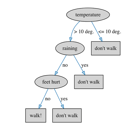
Decision trees are a popular technique for knowledge discovery because the model they produce (a tree) is a structure that is very easy for humans to interpret. In fact, we use decision trees internally in our everyday decision making. For example, when deciding whether to walk to work (rather than take the car) we might ask ourselves a series of questions like so:

Q: What is the temperature outside?

A: Greater than 10 degrees Celsius.

Q: OK, is it raining?

A: No, that's good.

Q: Are my feet hurting too much from yesterday's walk to work?

A: Yes - doh! Oh well, take the car it is then.

Graphically, this decision tree would look like the following diagram. To make a decision whether to walk to work or not, we start at the top (root) of the tree and consider the question at each interior node (ellipse). The answer to each question determines the branch of the tree to take. Leaves (rectangles) in the tree are the final decisions. Each path from root to leaf can also be thought of as an if-then rule, where the conditions (ellipses) are combined by AND operators.

Learning Decision Trees

We can think about the goal of the learning process for a decision tree as one that tries to find a way of segmenting the training data such that each segment contains only instances (rows) of one of the class labels. In the example above, we had only two class labels (decision outcomes): walk to work and don't walk to work. However, decision trees are equally capable of working with data that contains more than two classes - that is, multi-class problems. For all but simple problems, it is unlikely that we will find segments that contain instances of only one class, unless we build the decision tree such that each segment contains only one instance! Even then, depending on the type of input attributes it might not be possible to do this. Furthermore, such a strategy is unlikely to fit new data (that we haven't seen in the training data) very well.

In practice, decision trees employ a strategy that prefers segments that are as pure as possible, that is, they contain a strong majority of one class label. A number of methods for measuring purity have been explored in the machine learning field. One of the most popular is based on the field of information theory and, in particular, the concept of entropy. Once we have a way of measuring purity then constructing a decision tree boils down to finding the best attribute to split (segment) the data on. Nominal attributes naturally produce a segment (and branch in the tree) that corresponds to each distinct value of that attribute. For numeric attributes, a split point is found, such as for the temperature attribute at the root of the tree above. In both cases, splitting results in two or more segments; and the best attribute to use is the one that results in the best overall purity score across its segments. This splitting procedure is then repeated recursively for each subset or segment of instances.

The last part of the decision tree learning process is called pruning. As mentioned earlier, we can continue to expand the tree until we reach a point where the leaves contain only one instance. However, this is not likely to perform very well when predicting new date because the tree has overfit the training data. Real data is rarely clean cut and often contains noise, ambiguity and contradiction. Overfitting is when the model accounts for these factors. The solution is to limit how closely the tree fits the training data by either stopping the tree splitting process early, or by fully growing the tree and then chopping off branches that are not statistically warranted. The former is called pre-pruning, and the latter is called post-pruning. In practice, post-pruning gives better results because the full tree is generated and considered when removing branches. Pre-pruning, while computationally less expensive, runs the risk of stopping too early, and therefore missing important structure.

Strengths

• Basic algorithm is reasonably simple to implement
• Considers attribute dependencies
• Easy for humans to understand how predictions are made
• Can be made more powerful (at the expense of interpretability) via ensemble learning

Weaknesses

• Suffers from the data fragmentation problem when there are nominal attributes with many distinct values
• Can produce very large trees, which reduces interpretability
• Splitting criteria tend to be sensitive, and small changes in the data can result in large changes in the tree structure

 

Model interpretability: high

Common uses

As mentioned earlier, decision trees are often employed when a goal of learning is to gain insight into the data through the workings of the model. The tree structure of the model also lends itself to explaining how a given prediction is made. This is useful for obtaining model acceptance from stakeholders, such as problem domain experts, as they can compare the decision procedure in the tree to their own problem reasoning. While decision trees have reasonably good predictive performance in and of themselves, they really shine when many trees are learned and then combined together into an ensemble. Some of the most accurate machine learning models are based on ensembles of trees. Unfortunately, the added predictive accuracy comes at the expense of model interpretability, as a given data point is passed through multiple trees to produce a prediction.

Configuration

Decision tree algorithms usually have a set of default parameter settings that work well on a variety of problems. For those methods that implement pre-pruning, the most important parameter that the user might consider adjusting is that of tree depth. This indicates how many levels (or decisions) an instance passes through before reaching a leaf of the tree. Choosing too small a depth might result in the tree being too simple and failing to capture the structure of the problem in enough detail. Too large a value can result in overfitting, where spurious details of the training data get represented in the model. Trial and error, through experimentation, is the best way to find a good depth setting for a given problem. Algorithms that implement post-pruning tend to have a parameter that adjusts the sensitivity of the statistical test/heuristic that determines whether a branch will be removed or not. Again, default settings usually work very well.

Another option that is often available in decision tree algorithms is that of the (im)purity metric that is used in the recursive splitting procedure. However, experiments have shown that decision trees are far less sensitive to this setting than they are to the pruning strategy employed.

Example

Let's return to the simple weather dataset from the naïve Bayes section:

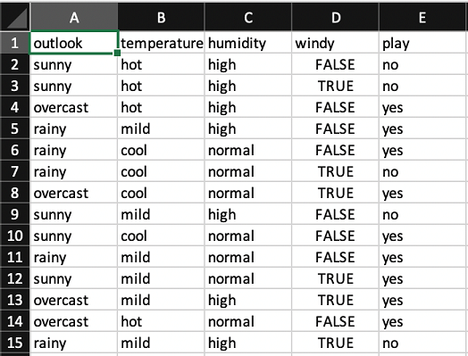
If we build Weka's J48 decision tree (with default parameter settings) on this dataset then we obtain the following decision tree:

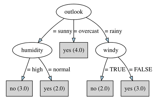
The first thing that we can see from this tree is that outlook is the most important attribute in the data for determining (i.e., deciding) the class label. Note that the attribute chosen at the root of the tree is always the most discriminatory across the entire dataset. In this case, the branch corresponding to outlook=overcast, by itself, accounts for four of the 14 instances in the dataset. The numbers in parentheses show how many training instances reach that leaf in the tree. If there are classification errors (i.e., instances with class labels that differ from the majority class at the leaf), then these are shown as a second number following a slash symbol in the parenthesis. In this tree for the weather data, we can see that every leaf is pure - that is, there are no misclassifications made. Furthermore, the entire dataset can be represented by three of the four attributes: outlook, humidity and windy. Temperature is not needed in order to correctly classify every example. In this way, the tree model can be thought of as a compressed representation of the input data.